Smoothed Differentiation¶

Experimental

Smoothed differentiation is experimental and currently supports problems with zero and nonnegative cones only (LPs and QPs). Support for SOC, exponential, and power cones is planned.

When differentiating through a conic solver, the gradients can be discontinuous at points where the active set changes (e.g., a constraint switches between active and inactive). Smoothed differentiation addresses this by computing gradients from a nearby point on the central path rather than the exact solution, producing smooth gradient curves that are better behaved for gradient-based optimization.

Usage¶

Enable smoothed differentiation via IPMSettings:

import moreau

settings = moreau.Settings(
    enable_grad=True,
    ipm_settings=moreau.IPMSettings(
        diff_method='smoothed',
        diff_smoothing_mu=1e-4,   # smoothing level (default)
    ),
)

The diff_smoothing_mu parameter controls the amount of smoothing. Larger values produce smoother gradients at the cost of accuracy relative to the exact solution; smaller values are closer to the exact (possibly discontinuous) gradients.

This works with all Moreau APIs: NumPy backward(), PyTorch autograd, and JAX grad.

PyTorch¶

from moreau.torch import Solver

solver = Solver(
    n=n, m=m,
    P_row_offsets=P_ro, P_col_indices=P_ci,
    A_row_offsets=A_ro, A_col_indices=A_ci,
    cones=cones,
    settings=moreau.Settings(
        ipm_settings=moreau.IPMSettings(
            diff_method='smoothed',
            diff_smoothing_mu=1e-3,
        ),
    ),
)

solver.setup(P_values, A_values)
solution = solver.solve(q, b)
solution.x.sum().backward()  # smooth gradients

JAX¶

import jax
from moreau.jax import Solver

solver = Solver(
    n=n, m=m,
    P_row_offsets=P_ro, P_col_indices=P_ci,
    A_row_offsets=A_ro, A_col_indices=A_ci,
    cones=cones,
    settings=moreau.Settings(
        ipm_settings=moreau.IPMSettings(
            diff_method='smoothed',
            diff_smoothing_mu=1e-3,
        ),
    ),
)

grad_fn = jax.grad(lambda q: solver.solve(P_data, A_data, q, b).x.sum())
dq = grad_fn(q)  # smooth gradients

Effect of Smoothing¶

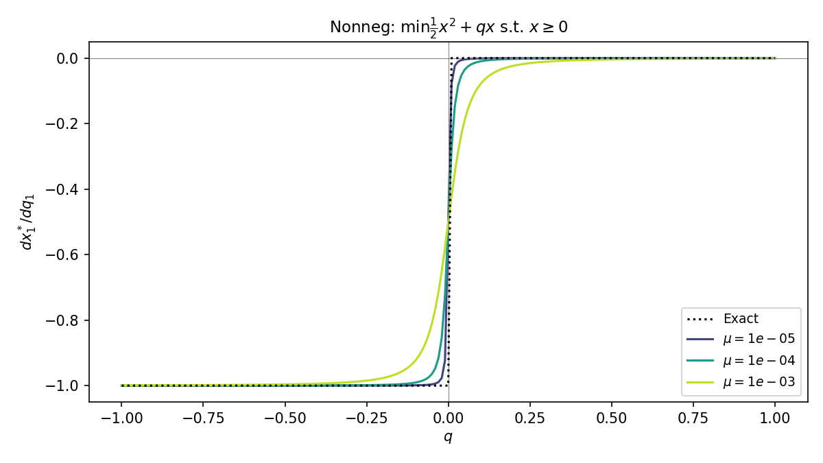
The plot below shows how smoothed differentiation affects the gradient \(\partial x^* / \partial q\) for a simple nonnegative-cone problem. The problem is parameterized by a scalar \(q\) that sweeps through a non-differentiable point (where the active set changes). The exact gradient (dashed black) has a sharp discontinuity; the smoothed gradients (colored curves) replace this with a smooth transition. Larger \(\mu\) produces more smoothing.

Nonnegative Cone¶

\[\min \; \tfrac{1}{2}x^2 + qx \quad \text{s.t.} \quad x \geq 0\]

How It Works¶

The standard (exact) backward pass differentiates the KKT conditions and uses the Jacobian \(H = D\Pi_{\mathcal{K}^*}(u)\) of the dual cone projection. This Jacobian is discontinuous at cone boundaries.

Smoothed differentiation replaces \(H\) with

\[H_\mu = \bigl(I + \mu \nabla^2 \varphi^*(z_\mu)\bigr)^{-1}\]

where \(\varphi^*\) is the dual barrier function and \(z_\mu\) is a point on the central path with average complementarity \(\mu\). This operator is \(C^\infty\) in both \(\mu\) and the problem data.

Obtaining the smoothing iterate¶

After the IPM converges to a high-accuracy solution, Moreau performs post-convergence refinement: it walks the complementarity \(\mu\) back up from \(\approx 0\) to \(\mu_\text{target}\) using pure centering steps. This produces an iterate that is approximately on the central path (near-feasible with the desired complementarity level) without affecting the forward solution quality.

The refinement typically takes 2–3 additional KKT factorizations, adding 30–50% overhead relative to the base solve. This cost is modest relative to the backward pass itself, which also requires a KKT factorization.

Settings Reference¶

Parameter	Default	Description
`diff_method`	`'auto'`	`'auto'`, `'exact'`, or `'smoothed'`. Auto selects exact.
`diff_smoothing_mu`	`1e-4`	Target smoothing level. Larger = smoother.
`diff_smoothing_step_factor`	`30.0`	Controls how aggressively each refinement step increases \(\mu\).

These are set on IPMSettings and passed to Settings:

settings = moreau.Settings(
    enable_grad=True,
    ipm_settings=moreau.IPMSettings(
        diff_method='smoothed',
        diff_smoothing_mu=1e-3,
    ),
)

When to Use Smoothed Differentiation¶

Use smoothed when:

Training with gradient descent and the loss landscape has kinks from active-set changes
Gradients are noisy or jumpy and you want a stabilizing effect
You need gradients that vary continuously with problem parameters

Use exact (default) when:

You need the most accurate gradients possible
Your problem parameters don’t cross active-set boundaries during optimization
You’re computing sensitivities rather than training

Limitations¶

Currently supports zero and nonnegative cones only (LPs and QPs). Using diff_method='smoothed' with SOC, exponential, or power cones will raise an error. If you need smoothed differentiation for other cone types, please contact us.
Adds overhead from post-convergence refinement iterations (typically 30–50%).